VisLies 2018 Gallery
October 23, 2018
What a great year for VisLies! We had a small room, but we packed it. And you guys brought some great examples for us.
Let’s take a look at all the great lies everyone told.
Recalibrate Your Banan-o-meter
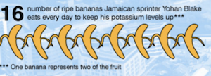
Ken Moreland started us off with a level of silliness measured in bananas. This infographic tells us a bit of trivia about the number of bananas consumed daily by sprinter Yohan Blake. But a closer look reveals that the number and the image don’t quite add up.
The graphic shows 8 bananas, but Yohan eats an even more impressive 16. What gives? Well, if you look closely, you will see a note that “One banana represents two of the fruit.”
Why does 1 banana equal 2? You need to recalibrate your banan-o-meter. If you want to impress people with your bananas, just show them your bananas.
A Lonely Bar
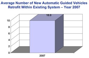
Ken next showed this use, or rather misuse, of a bar chart. This appears to be an attempt to make the presentation of a single dull number more interesting and failing in multiple ways.
To start with, someone has clearly turned on the 3D bar chart capabilities in Excel, which is something that we generally discourage. But the problem with 3D representations is that they make it more difficult to understand the relative position of things in space. For example, the top of this bar is aligned with both the 8 and 10 ticks.
But the really weird part of this display is that it is a lone bar. The point of a bar chart is to visually compare the relative value of two or more values. But this number is not compared to anything. It looks big, but any number would look big when you scale the bar to fit the space. Retrofitting 10 cars might actually be low if that is all you did all year.
Helpings of Pie
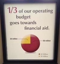
It is no secret that Ken is not a fan of pie charts, and so he often provides examples of their use and abuse. First up is this public display where the pie chart is essentially correct, but the designer apparently does not know what one quarter looks like.

Unlike Ken, news organizations tend to like pie charts very much, and apparently they like abusing them as well. Here is a bizarre example of a pie chart that contains more than 100% of content. It’s a paradox how the pie chart contains more pie than the pie chart contains. Perhaps the designers were ingesting some of the material they were talking about.
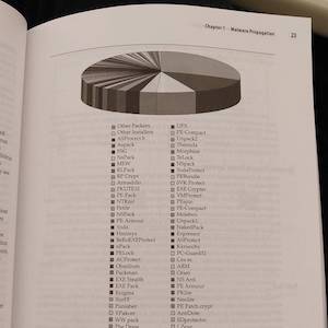
This final bar chart is fraught with problems. The biggest problem by far is that there are way too many wedges to keep track of. Just to make sure there is no possible way to understand what is going on, the chart is printed without color. The designers of this chart must hate their data.
Email by the Billions
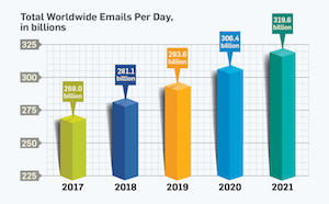
Ken showed us this plot that comes from a recent technical paper. The chart clearly puts form over function with the needless 3D effects and shadows (which are inconsistent).
But the more serious issue is that the plot unfairly represents the data. The intention of this chart is clearly to demonstrate that email traffic is steeply on the rise. But does the data agree with that?
If we look closely, we see that the bars do not start at 0. Instead, they start at a very large 225 billion emails.

This plot corrects the scaling. In the previous plot it appears that the amount of email traffic has doubled, but in truth email traffic is only going up by a small fraction in this time.
Speaking of time, the time range selected for this plot is a bit weird, too. The time range of the plot is fairly narrow. The majority of the plot is a prediction of the future. Why not show the trend with collected data?
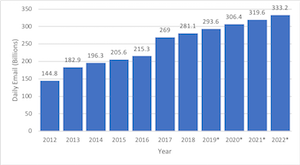
Ken figures that the data for this plot comes from the Radicati Group. In about an hour, Ken was able to pull data back to 2012. here is the plot of that data.
As you can see, there have been some recent surges in email traffic, but the look like they may be leveling off. Again, not the story of extreme email traffic growth purported by the original chart.
Surprise Results
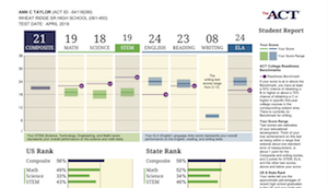
Earlier this year, Ken’s daughter took the ACT, an aptitude test commonly used for admissions by may United States colleges. When she received her results, which were similar to the example shown here, she received a shock. Although most of the scores were as expected, the score for writing (second column from the right) was shockingly low.
Did she fail that part of the test? Actually, no. It is a simple matter of odd scaling. Most of the sections in the ACT as well as the composite scores are graded on a scale from 1 to 36. But for some reason the writing test scores are scaled from 2 to 12. Because the scaling range is so much smaller than all other scores, it becomes a scary shock for each and every of the 1.7 million students that take the test every year.
The problem is simple to solve. Just rescale the writing score to be in the 36 point scale as the others (multiply the score by 3).
Farewell Georges

It is with a heavy heart this year that we say goodbye to Georges Grinstein. Georges was one of the founding members of the first VisLies (in 1995!) and had continued to help organize VisLies since. Unfortunately, Georges passed away this year.
We spend some time this year to remember Georges and celebrate his life.
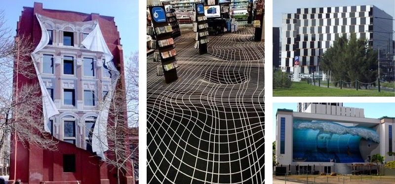
Something that Georges enjoyed doing each year at VisLies was presenting an example of an (intentional) optical illusion in the form of architecture. Above are some examples of the kinds of things Georges showed.
Ken choose to honor Georges by showing his own personal favorite illusion in architecture. This example comes from a set of the biggest lying liars who have been operating for decades: the Walt Disney park Imagineers.
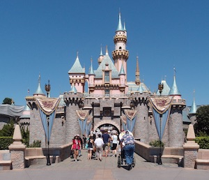
Walt Disney and his Imagineers are some of the biggest liars you will ever meet. Just about everything you look at in one of the Walt Disney parks is a big fat lie. Take, for example, the iconic Sleeping Beauty Castle at the center of the Disneyland park shown here. The top of this faux castle reaches about 77 feet (23 meters), which is not exactly low but is barely 1/3 the height of the Neuschwanstein Castle on which it is based. Instead, the architecture uses numerous examples of forced perspective to make it appear taller. Pay particular attention to the turrets. The ones at the base of the castle are quite wide, but the tend to get thinner as you move up the castle, making them appear to be further away.
Lake Macquarie Got Bigger
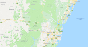
Ben Simons started with a quick geography lesson of Sydney, Australia. Not that there is any specific lie about Sydney, but as a quick orientation for us Northern-Hemisphere-ers that might not be familiar with it. The map is shown here. As you can see, the coast has its fair share of bays and rivers, but otherwise follows an arc.
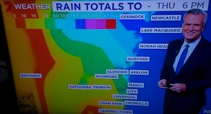
So, Ben was a bit surprised when he looked up to this TV weather report and saw a rather startling change in the coastline. According to this map, lake Macquarie (labeled near the weatherperson’s head) has become huge.
After a double take, it starts to become clear that, no, a huge chunk of Australia has not broken off to sea. Yet. Probably. Rather, the colors used to represent rainfall unwisely use the same color to represent ocean in this map.
Rules of probability dictate that the area in this map between the Cessnock and Lake Macquarie labels has just received between 150 and 200mm of rain (which is probably not enough to turn the whole area into a lake). But what about the other patches? What about the other subtle features of the map? Or are maybe we are supposed to assume that it’s just really rainy off the coast?
The ineptitude of the colors keeps on giving. The colors are thoughtlessly picked from rainbow hues, which is a common target of VisLies. To make matters worse, the color red is for some reason featured twice and there are two very similar shades of orange. The order of the colors is also confusing: orange, red, orange, yellow, lime…? Even more confusing, there is something odd with a green region just north of Katoomba and west of Richmond. That area has a yellow-green color that is featured nowhere in the discrete colors of the scale.
Additionally, the intervals on the color map’s legend increase unpredictably: 1, 5, 10, 15, 25, 50, 100, 150, 200, 300, 400. It goes up in 5’s, then one step of 10, then one 25, three 50’s, and two 100’s, doubling at arbitrary points. How is one to make sense of the progression?
And what is happening with the weird texture pattern in the lower left? Did they run out of orange pixels?
This is a map that keeps on giving… confusion!
Evil Histograms
Michael Correll brought up the positive and negative aspects of histogram visualizations. Histograms are a good way to show the distribution of data. However, continuous data must be grouped into bins of defined ranges.
And therein lies a problem. The choice of bins can have a large effect on what the visualization shows. To demonstrate this, Michael showed an adversarial visualization application that attempts to make the most evil histograms possible.
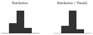
Here is an example generated by the application. The histogram on the left was generated from a set of 100 data values randomly generated from a Gaussian probability distribution. The histogram on the right was generated from the same 100 values plus an additional 20 data items with the same value, which should really skew the apparent distribution. However the bins being used for this histogram make the two look nearly identical.
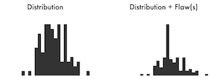
In contrast, consider these two histograms. The underlying data of these two histograms is exactly the same as the previous example. But in this case the different bin choices highlight the dissimilarity between the two data sets (although you might be hard pressed to realize the exact relationship between the two sets of data).
In general, fewer bins (with wider ranges) tend to hide details. That would suggest that having more bins is better, but too many bins (with narrow ranges) can fail to estimate the density of the samples. Consequently, when using histogram visualizations it is prudent to experiment with the number of bins to best understand the data.
Deceitful Backgrounds

David Borland presented a fun and relevant optical illusion named simultaneous contrast in which the background can have a dramatic effect on the perceived colors in it. Take, for example, the bar shown here. The bar is clearly lighter on its left end and darker on its right end, right? Well, no. The bar is actually a uniform color, but it appears to change color because of the changing background. Don’t believe it? Cover the top and bottom of the bar with your hands and you can see the uniform color. Now remove your hands. Even knowing the bar is all one color, it is still hard to “see” it as one color.
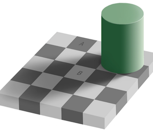
The effects of simultaneous contrast can be very dramatic. Take for
example this image and look particularly at the tiles marked A and B.
A is clearly darker than B, right? Well, actually, the pixel color
value of both is the same. (It’s hex color #8B8B8B or 47% grayscale. Don’t
believe us? Check the colors with your favorite image editor. Go ahead.
We’ll wait.) But regardless of how much you tell yourself that the two
colors are the same, you just can’t “see” them the same.
Beware, because simultaneous contrast can come into play in visualization. Human viewers might not see colors with the same brightness that they are actually displayed. This helps explain why studies show subjects error up to 20% when using grayscale-only representations for values.
Bars with no Basis
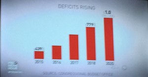
If bars are not scaled, is it really a chart? Richard Johansen was watching PBS one day and came across this bar chart, which did not look right. Something did no look right, so he quickly took a picture, printed it out, and measured the length of the bars. Sure enough, none of the scales of any of the bars matched each other.
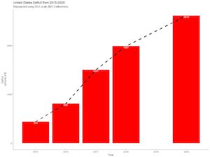
If you take the scale from the reported number of the 2015 bar and use that to derive numbers for the other bars as Richard did, you get a chart that looks like this.
Note that these rescaled numbers are way off the actual values reported in the original chart.
If you also add the space for the missing 2019 value, as is done here, you see that the growth of the bars actually slows down toward the end.
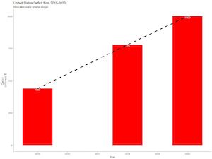
Modifying again to take the values reported in the original bar chart and scaling the bars on that, you get a chart like this one here. Missing are the bars where concrete numbers were not given as we can only guess what the actual values are supposed to be. Interestingly, the properly scaled bars shows a linear increase that was somehow also shown in the original plot even though the the time scale got compressed at the end. The original chart appears to have lied so much that it has somehow stumbled back into the general vicinity of truth.